What Is The Size Of A Hydrogen Atom In Meters?

Cantlet of the element hydrogen

This article is virtually the physics of the hydrogen atom. For a chemical description, see hydrogen. For monatomic hydrogen, see Hydrogen § Diminutive hydrogen.

Hydrogen cantlet,¹H

General
Symbol	iH
Names	hydrogen cantlet, H-ane, protium
Protons (Z)	one
Neutrons (North)	0
Nuclide data
Natural abundance	99.985%
One-half-life (t i/two)	stable
Isotope mass	1.007825 u
Spin	one / ii
Excess energy	vii288.969±0.001 keV
Binding free energy	0.000±0.0000 keV
Isotopes of hydrogen Complete table of nuclides

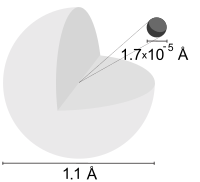
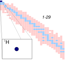
Depiction of a hydrogen atom showing the diameter as most twice the Bohr model radius. (Prototype not to calibration)

A hydrogen cantlet is an atom of the chemical element hydrogen. The electrically neutral atom contains a single positively charged proton and a unmarried negatively charged electron leap to the nucleus past the Coulomb force. Atomic hydrogen constitutes virtually 75% of the baryonic mass of the universe.^[1]

In everyday life on Earth, isolated hydrogen atoms (called "atomic hydrogen") are extremely rare. Instead, a hydrogen cantlet tends to combine with other atoms in compounds, or with another hydrogen cantlet to form ordinary (diatomic) hydrogen gas, H₂. "Diminutive hydrogen" and "hydrogen atom" in ordinary English use have overlapping, yet singled-out, meanings. For example, a water molecule contains two hydrogen atoms, merely does non comprise diminutive hydrogen (which would refer to isolated hydrogen atoms).

Diminutive spectroscopy shows that at that place is a discrete infinite set of states in which a hydrogen (or whatsoever) cantlet can exist, opposite to the predictions of classical physics. Attempts to develop a theoretical understanding of the states of the hydrogen atom have been important to the history of quantum mechanics, since all other atoms can exist roughly understood by knowing in detail nearly this simplest atomic structure.

Isotopes [edit]

The almost abundant isotope, hydrogen-1, protium, or lite hydrogen, contains no neutrons and is but a proton and an electron. Protium is stable and makes up 99.985% of naturally occurring hydrogen atoms.^[2]

Deuterium contains one neutron and 1 proton in its nucleus. Deuterium is stable and makes up 0.0156% of naturally occurring hydrogen^[2] and is used in industrial processes like nuclear reactors and Nuclear Magnetic Resonance.

Tritium contains two neutrons and one proton in its nucleus and is not stable, decomposable with a half-life of 12.32 years. Because of its short half-life, tritium does non be in nature except in trace amounts.

Heavier isotopes of hydrogen are just created artificially in particle accelerators and have half-lives on the society of 10⁻²² seconds. They are unbound resonances located beyond the neutron drip line; this results in prompt emission of a neutron.

The formulas beneath are valid for all three isotopes of hydrogen, but slightly different values of the Rydberg constant (correction formula given below) must be used for each hydrogen isotope.

Hydrogen ion [edit]

Solitary neutral hydrogen atoms are rare under normal weather. Nonetheless, neutral hydrogen is common when it is covalently leap to another atom, and hydrogen atoms can also exist in cationic and anionic forms.

If a neutral hydrogen cantlet loses its electron, information technology becomes a cation. The resulting ion, which consists solely of a proton for the usual isotope, is written as "H⁺" and sometimes chosen hydron. Costless protons are common in the interstellar medium, and solar wind. In the context of aqueous solutions of classical Brønsted–Lowry acids, such every bit hydrochloric acid, it is really hydronium, H₃O⁺, that is meant. Instead of a literal ionized unmarried hydrogen atom being formed, the acid transfers the hydrogen to H_twoO, forming H_threeO⁺.

If instead a hydrogen atom gains a 2d electron, it becomes an anion. The hydrogen anion is written as "H^–" and called hydride.

Theoretical assay [edit]

The hydrogen cantlet has special significance in breakthrough mechanics and quantum field theory as a elementary two-body problem physical system which has yielded many simple analytical solutions in closed-course.

Failed classical description [edit]

Experiments by Ernest Rutherford in 1909 showed the construction of the atom to be a dumbo, positive nucleus with a tenuous negative accuse deject around information technology. This immediately raised questions about how such a system could exist stable. Classical electromagnetism had shown that any accelerating charge radiates energy, every bit shown by the Larmor formula. If the electron is assumed to orbit in a perfect circle and radiates energy continuously, the electron would rapidly spiral into the nucleus with a fall time of:^[three]

$${\displaystyle t_{\text{fall}}\approx {\frac {a_{0}^{three}}{4r_{0}^{2}c}}\approx 1.half-dozen\times 10^{-11}{\text{ s}},}$$

where ${\displaystyle a_{0}}$ is the Bohr radius and ${\displaystyle r_{0}}$ is the classical electron radius. If this were true, all atoms would instantly collapse, however atoms seem to be stable. Furthermore, the spiral inward would release a smear of electromagnetic frequencies as the orbit got smaller. Instead, atoms were observed to simply emit discrete frequencies of radiation. The resolution would lie in the development of quantum mechanics.

Bohr–Sommerfeld Model [edit]

In 1913, Niels Bohr obtained the energy levels and spectral frequencies of the hydrogen cantlet after making a number of simple assumptions in club to correct the failed classical model. The assumptions included:

1. Electrons can but be in certain, discrete circular orbits or stationary states, thereby having a detached ready of possible radii and energies.
2. Electrons do not emit radiation while in ane of these stationary states.
3. An electron tin gain or lose energy by jumping from one detached orbit to another.

Bohr supposed that the electron's angular momentum is quantized with possible values:

$${\displaystyle Fifty=north\hbar }$$

where ${\displaystyle n=1,2,3,\ldots }$ and ${\displaystyle \hbar }$ is Planck constant over ${\displaystyle ii\pi }$ . He as well supposed that the centripetal forcefulness which keeps the electron in its orbit is provided by the Coulomb forcefulness, and that energy is conserved. Bohr derived the energy of each orbit of the hydrogen atom to be:^[4]

$${\displaystyle E_{north}=-{\frac {m_{eastward}eastward^{4}}{2(four\pi \varepsilon _{0})^{two}\hbar ^{two}}}{\frac {1}{due north^{2}}},}$$

where ${\displaystyle m_{e}}$ is the electron mass, ${\displaystyle e}$ is the electron charge, ${\displaystyle \epsilon _{0}}$ is the vacuum permittivity, and ${\displaystyle north}$ is the quantum number (now known as the principal quantum number). Bohr's predictions matched experiments measuring the hydrogen spectral series to the outset order, giving more confidence to a theory that used quantized values.

For ${\displaystyle n=ane}$ , the value^[five]

$${\displaystyle {\frac {m_{eastward}eastward^{4}}{two(4\pi \varepsilon _{0})^{two}\hbar ^{2}}}={\frac {m_{\text{e}}e^{4}}{8h^{two}\varepsilon _{0}^{two}}}=1\,{\text{Ry}}=13.605\;693\;122\;994(26)\,{\text{eV}}}$$

is called the Rydberg unit of energy. It is related to the Rydberg constant ${\displaystyle R_{\infty }}$ of atomic physics past ${\displaystyle ane\,{\text{Ry}}\equiv hcR_{\infty }.}$

The exact value of the Rydberg constant assumes that the nucleus is infinitely massive with respect to the electron. For hydrogen-i, hydrogen-2 (deuterium), and hydrogen-3 (tritium) which have finite mass, the constant must be slightly modified to use the reduced mass of the system, rather than simply the mass of the electron. This includes the kinetic energy of the nucleus in the problem, because the total (electron plus nuclear) kinetic energy is equivalent to the kinetic energy of the reduced mass moving with a velocity equal to the electron velocity relative to the nucleus. However, since the nucleus is much heavier than the electron, the electron mass and reduced mass are about the same. The Rydberg constant R_Grand for a hydrogen atom (one electron), R is given past

$${\displaystyle R_{M}={\frac {R_{\infty }}{1+m_{\text{e}}/M}},}$$

where ${\displaystyle Grand}$ is the mass of the atomic nucleus. For hydrogen-one, the quantity ${\displaystyle m_{\text{due east}}/M,}$ is nearly 1/1836 (i.due east. the electron-to-proton mass ratio). For deuterium and tritium, the ratios are about i/3670 and 1/5497 respectively. These figures, when added to 1 in the denominator, represent very pocket-size corrections in the value of R, and thus just pocket-size corrections to all energy levels in respective hydrogen isotopes.

There were however problems with Bohr'southward model:

1. it failed to predict other spectral details such every bit fine structure and hyperfine structure
2. it could only predict free energy levels with whatsoever accuracy for single–electron atoms (hydrogen–like atoms)
3. the predicted values were only correct to ${\displaystyle \alpha ^{two}\approx 10^{-five}}$ , where ${\displaystyle \alpha }$ is the fine-structure constant.

Most of these shortcomings were resolved by Arnold Sommerfeld's modification of the Bohr model. Sommerfeld introduced two additional degrees of freedom, allowing an electron to movement on an elliptical orbit characterized past its eccentricity and declination with respect to a called axis. This introduced two additional breakthrough numbers, which correspond to the orbital angular momentum and its projection on the called centrality. Thus the right multiplicity of states (except for the factor two accounting for the nevertheless unknown electron spin) was found. Further, by applying special relativity to the elliptic orbits, Sommerfeld succeeded in deriving the right expression for the fine structure of hydrogen spectra (which happens to be exactly the same as in the most elaborate Dirac theory). However, some observed phenomena, such as the anomalous Zeeman effect, remained unexplained. These issues were resolved with the total development of quantum mechanics and the Dirac equation. Information technology is often alleged that the Schrödinger equation is superior to the Bohr–Sommerfeld theory in describing hydrogen atom. This is not the case, as most of the results of both approaches coincide or are very close (a remarkable exception is the problem of hydrogen atom in crossed electric and magnetic fields, which cannot be self-consistently solved in the framework of the Bohr–Sommerfeld theory), and in both theories the main shortcomings effect from the absenteeism of the electron spin. It was the complete failure of the Bohr–Sommerfeld theory to explicate many-electron systems (such as helium atom or hydrogen molecule) which demonstrated its inadequacy in describing quantum phenomena.

Schrödinger equation [edit]

The Schrödinger equation allows one to calculate the stationary states and also the time evolution of breakthrough systems. Exact belittling answers are available for the nonrelativistic hydrogen atom. Before we go to present a formal account, here we give an elementary overview.

Given that the hydrogen atom contains a nucleus and an electron, quantum mechanics allows one to predict the probability of finding the electron at whatever given radial altitude ${\displaystyle r}$ . Information technology is given by the square of a mathematical function known equally the "wavefunction," which is a solution of the Schrödinger equation. The everyman energy equilibrium land of the hydrogen cantlet is known as the ground state. The ground state wave function is known as the ${\displaystyle 1\mathrm {s} }$ wavefunction. It is written as:

$${\displaystyle \psi _{1\mathrm {s} }(r)={\frac {1}{{\sqrt {\pi }}a_{0}^{3/2}}}east^{-r/a_{0}}.}$$

Here, ${\displaystyle a_{0}}$ is the numerical value of the Bohr radius. The probability density of finding the electron at a distance ${\displaystyle r}$ in whatsoever radial direction is the squared value of the wavefunction:

$${\displaystyle |\psi _{1\mathrm {south} }(r)|^{2}={\frac {one}{\pi a_{0}^{3}}}eastward^{-2r/a_{0}}.}$$

The ${\displaystyle 1\mathrm {south} }$ wavefunction is spherically symmetric, and the surface area of a trounce at distance ${\displaystyle r}$ is ${\displaystyle 4\pi r^{2}}$ , so the total probability ${\displaystyle P(r)\,dr}$ of the electron beingness in a shell at a distance ${\displaystyle r}$ and thickness ${\displaystyle dr}$ is

$${\displaystyle P(r)\,dr=4\pi r^{2}|\psi _{one\mathrm {s} }(r)|^{2}\,dr.}$$

It turns out that this is a maximum at ${\displaystyle r=a_{0}}$ . That is, the Bohr picture of an electron orbiting the nucleus at radius ${\displaystyle a_{0}}$ corresponds to the well-nigh probable radius. Actually, there is a finite probability that the electron may be found at whatever identify ${\displaystyle r}$ , with the probability indicated by the square of the wavefunction. Since the probability of finding the electron somewhere in the whole volume is unity, the integral of ${\displaystyle P(r)\,dr}$ is unity. And then we say that the wavefunction is properly normalized.

As discussed below, the ground state ${\displaystyle one\mathrm {s} }$ is also indicated by the quantum numbers ${\displaystyle (n=one,\ell =0,m=0)}$ . The second lowest energy states, but above the ground state, are given past the quantum numbers ${\displaystyle (2,0,0)}$ , ${\displaystyle (2,1,0)}$ , and ${\displaystyle (2,i,\pm i)}$ . These ${\displaystyle northward=2}$ states all have the same energy and are known as the ${\displaystyle 2\mathrm {due south} }$ and ${\displaystyle ii\mathrm {p} }$ states. There is one ${\displaystyle 2\mathrm {s} }$ state:

$${\displaystyle \psi _{2,0,0}={\frac {i}{4{\sqrt {two\pi }}a_{0}^{iii/2}}}\left(2-{\frac {r}{a_{0}}}\right)e^{-r/2a_{0}},}$$

and in that location are iii ${\displaystyle ii\mathrm {p} }$ states:

$${\displaystyle \psi _{ii,1,0}={\frac {one}{iv{\sqrt {two\pi }}a_{0}^{iii/2}}}{\frac {r}{a_{0}}}due east^{-r/2a_{0}}\cos \theta ,}$$

$${\displaystyle \psi _{two,1,\pm ane}=\mp {\frac {1}{8{\sqrt {\pi }}a_{0}^{iii/two}}}{\frac {r}{a_{0}}}e^{-r/2a_{0}}\sin \theta ~e^{\pm i\varphi }.}$$

An electron in the ${\displaystyle ii\mathrm {s} }$ or ${\displaystyle 2\mathrm {p} }$ state is most likely to exist constitute in the 2d Bohr orbit with energy given by the Bohr formula.

Wavefunction [edit]

The Hamiltonian of the hydrogen atom is the radial kinetic energy operator and Coulomb attraction strength between the positive proton and negative electron. Using the time-independent Schrödinger equation, ignoring all spin-coupling interactions and using the reduced mass ${\displaystyle \mu =m_{e}M/(m_{due east}+M)}$ , the equation is written as:

$${\displaystyle \left(-{\frac {\hbar ^{two}}{2\mu }}\nabla ^{2}-{\frac {due east^{2}}{4\pi \varepsilon _{0}r}}\correct)\psi (r,\theta ,\varphi )=Eastward\psi (r,\theta ,\varphi )}$$

Expanding the Laplacian in spherical coordinates:

$${\displaystyle -{\frac {\hbar ^{2}}{2\mu }}\left[{\frac {1}{r^{2}}}{\frac {\partial }{\fractional r}}\left(r^{2}{\frac {\partial \psi }{\partial r}}\right)+{\frac {one}{r^{two}\sin \theta }}{\frac {\fractional }{\partial \theta }}\left(\sin \theta {\frac {\partial \psi }{\partial \theta }}\right)+{\frac {one}{r^{2}\sin ^{2}\theta }}{\frac {\partial ^{2}\psi }{\fractional \varphi ^{2}}}\correct]-{\frac {e^{2}}{4\pi \varepsilon _{0}r}}\psi =Eastward\psi }$$

This is a separable, partial differential equation which can exist solved in terms of special functions. When the wavefunction is separated as product of functions ${\displaystyle R(r)}$ , ${\displaystyle \Theta (\theta )}$ , and ${\displaystyle \Phi (\varphi )}$ iii contained differential functions appears^[6] with A and B being the separation constants:

• radial:

  $${\displaystyle {\frac {d}{dr}}\left(r^{2}{\frac {dR}{dr}}\right)+{\frac {2\mu r^{2}}{\hbar ^{two}}}\left(Due east+{\frac {e^{2}}{iv\pi \varepsilon _{0}r}}\correct)R-AR=0}$$

  

• polar:

  $${\displaystyle {\frac {\sin \theta }{\Theta }}{\frac {d}{d\theta }}\left(\sin \theta {\frac {d\Theta }{d\theta }}\right)+A\sin ^{two}\theta -B=0}$$

  

• azimuth:

  $${\displaystyle {\frac {1}{\Phi }}{\frac {d^{2}\Phi }{d\varphi ^{ii}}}+B=0.}$$

  

The normalized position wavefunctions, given in spherical coordinates are:

$${\displaystyle \psi _{n\ell m}(r,\theta ,\varphi )={\sqrt {{\left({\frac {2}{na_{0}^{*}}}\correct)}^{3}{\frac {(n-\ell -1)!}{2n(n+\ell )!}}}}due east^{-\rho /2}\rho ^{\ell }L_{due north-\ell -1}^{two\ell +1}(\rho )Y_{\ell }^{m}(\theta ,\varphi )}$$

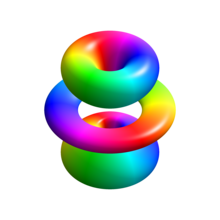
3D illustration of the eigenstate ${\displaystyle \psi _{four,3,1}}$ . Electrons in this state are 45% likely to exist found within the solid body shown.

where:

The breakthrough numbers tin take the following values:

• ${\displaystyle n=i,ii,iii,\ldots }$ (master quantum number)
• ${\displaystyle \ell =0,1,2,\ldots ,northward-1}$ (azimuthal breakthrough number)
• ${\displaystyle m=-\ell ,\ldots ,\ell }$ (magnetic quantum number).

Additionally, these wavefunctions are normalized (i.e., the integral of their modulus square equals ane) and orthogonal:

$${\displaystyle \int _{0}^{\infty }r^{2}\,dr\int _{0}^{\pi }\sin \theta \,d\theta \int _{0}^{2\pi }d\varphi \,\psi _{n\ell thou}^{*}(r,\theta ,\varphi )\psi _{northward'\ell 'm'}(r,\theta ,\varphi )=\langle northward,\ell ,m|n',\ell ',m'\rangle =\delta _{nn'}\delta _{\ell \ell '}\delta _{mm'},}$$

where ${\displaystyle |n,\ell ,k\rangle }$ is the land represented by the wavefunction ${\displaystyle \psi _{n\ell k}}$ in Dirac note, and ${\displaystyle \delta }$ is the Kronecker delta function.^[11]

The wavefunctions in momentum space are related to the wavefunctions in position space through a Fourier transform

$${\displaystyle \varphi (p,\theta _{p},\varphi _{p})=(two\pi \hbar )^{-iii/2}\int e^{-i{\vec {p}}\cdot {\vec {r}}/\hbar }\psi (r,\theta ,\varphi )\,dV,}$$

which, for the spring states, results in^[12]

$${\displaystyle \varphi (p,\theta _{p},\varphi _{p})={\sqrt {{\frac {2}{\pi }}{\frac {(northward-\ell -1)!}{(north+\ell )!}}}}n^{2}two^{2\ell +2}\ell !{\frac {north^{\ell }p^{\ell }}{(n^{two}p^{two}+i)^{\ell +two}}}C_{n-\ell -ane}^{\ell +1}\left({\frac {n^{2}p^{two}-1}{n^{2}p^{2}+1}}\right)Y_{\ell }^{yard}(\theta _{p},\varphi _{p}),}$$

where ${\displaystyle C_{N}^{\blastoff }(x)}$ denotes a Gegenbauer polynomial and ${\displaystyle p}$ is in units of ${\displaystyle \hbar /a_{0}^{*}}$ .

The solutions to the Schrödinger equation for hydrogen are analytical, giving a elementary expression for the hydrogen free energy levels and thus the frequencies of the hydrogen spectral lines and fully reproduced the Bohr model and went beyond it. It likewise yields two other quantum numbers and the shape of the electron'southward wave function ("orbital") for the diverse possible breakthrough-mechanical states, thus explaining the anisotropic character of diminutive bonds.

The Schrödinger equation besides applies to more complicated atoms and molecules. When there is more 1 electron or nucleus the solution is non analytical and either computer calculations are necessary or simplifying assumptions must be made.

Since the Schrödinger equation is only valid for non-relativistic quantum mechanics, the solutions information technology yields for the hydrogen atom are non entirely correct. The Dirac equation of relativistic quantum theory improves these solutions (see below).

Results of Schrödinger equation [edit]

The solution of the Schrödinger equation (wave equation) for the hydrogen atom uses the fact that the Coulomb potential produced by the nucleus is isotropic (it is radially symmetric in space and only depends on the distance to the nucleus). Although the resulting energy eigenfunctions (the orbitals) are non necessarily isotropic themselves, their dependence on the athwart coordinates follows completely generally from this isotropy of the underlying potential: the eigenstates of the Hamiltonian (that is, the free energy eigenstates) tin can be called as simultaneous eigenstates of the angular momentum operator. This corresponds to the fact that angular momentum is conserved in the orbital motion of the electron effectually the nucleus. Therefore, the energy eigenstates may exist classified by two angular momentum quantum numbers, ${\displaystyle \ell }$ and ${\displaystyle k}$ (both are integers). The athwart momentum quantum number ${\displaystyle \ell =0,1,2,\ldots }$ determines the magnitude of the angular momentum. The magnetic breakthrough number ${\displaystyle m=-\ell ,\ldots ,+\ell }$ determines the projection of the athwart momentum on the (arbitrarily chosen) ${\displaystyle z}$ -axis.

In addition to mathematical expressions for full angular momentum and angular momentum project of wavefunctions, an expression for the radial dependence of the wave functions must be establish. It is only here that the details of the ${\displaystyle 1/r}$ Coulomb potential enter (leading to Laguerre polynomials in ${\displaystyle r}$ ). This leads to a third quantum number, the principal quantum number ${\displaystyle northward=1,ii,iii,\ldots }$ . The master quantum number in hydrogen is related to the atom's total energy.

Annotation that the maximum value of the angular momentum quantum number is limited by the principal quantum number: it can run just up to ${\displaystyle n-1}$ , i.e., ${\displaystyle \ell =0,1,\ldots ,northward-1}$ .

Due to angular momentum conservation, states of the same ${\displaystyle \ell }$ but unlike ${\displaystyle m}$ have the aforementioned free energy (this holds for all problems with rotational symmetry). In addition, for the hydrogen atom, states of the same ${\displaystyle n}$ only unlike ${\displaystyle \ell }$ are also degenerate (i.e., they have the same energy). Still, this is a specific property of hydrogen and is no longer true for more complicated atoms which accept an (constructive) potential differing from the form ${\displaystyle ane/r}$ (due to the presence of the inner electrons shielding the nucleus potential).

Taking into account the spin of the electron adds a last breakthrough number, the projection of the electron's spin angular momentum forth the ${\displaystyle z}$ -axis, which can take on 2 values. Therefore, whatever eigenstate of the electron in the hydrogen atom is described fully by 4 quantum numbers. Co-ordinate to the usual rules of breakthrough mechanics, the actual state of the electron may exist whatever superposition of these states. This explains also why the choice of ${\displaystyle z}$ -axis for the directional quantization of the angular momentum vector is immaterial: an orbital of given ${\displaystyle \ell }$ and ${\displaystyle m'}$ obtained for another preferred centrality ${\displaystyle z'}$ tin always be represented equally a suitable superposition of the diverse states of dissimilar ${\displaystyle m}$ (but same ${\displaystyle \ell }$ ) that accept been obtained for ${\displaystyle z}$ .

Mathematical summary of eigenstates of hydrogen cantlet [edit]

In 1928, Paul Dirac found an equation that was fully compatible with special relativity, and (every bit a outcome) made the wave function a 4-component "Dirac spinor" including "up" and "down" spin components, with both positive and "negative" energy (or matter and antimatter). The solution to this equation gave the following results, more accurate than the Schrödinger solution.

Energy levels [edit]

The free energy levels of hydrogen, including fine structure (excluding Lamb shift and hyperfine structure), are given by the Sommerfeld fine structure expression:^[13]

$${\displaystyle {\begin{aligned}E_{j\,n}={}&-\mu c^{two}\left[1-\left(1+\left[{\frac {\alpha }{due north-j-{\frac {one}{2}}+{\sqrt {\left(j+{\frac {1}{ii}}\right)^{2}-\alpha ^{ii}}}}}\right]^{2}\right)^{-1/2}\right]\\\approx {}&-{\frac {\mu c^{ii}\alpha ^{2}}{2n^{ii}}}\left[i+{\frac {\blastoff ^{2}}{northward^{two}}}\left({\frac {n}{j+{\frac {ane}{2}}}}-{\frac {three}{4}}\correct)\correct],\terminate{aligned}}}$$

where ${\displaystyle \alpha }$ is the fine-construction abiding and ${\displaystyle j}$ is the total angular momentum quantum number, which is equal to ${\displaystyle \left|\ell \pm {\tfrac {ane}{2}}\right|}$ , depending on the orientation of the electron spin relative to the orbital angular momentum.^[14] This formula represents a pocket-sized correction to the energy obtained past Bohr and Schrödinger as given higher up. The cistron in square brackets in the terminal expression is almost one; the actress term arises from relativistic effects (for details, see #Features going beyond the Schrödinger solution). It is worth noting that this expression was first obtained past A. Sommerfeld in 1916 based on the relativistic version of the old Bohr theory. Sommerfeld has still used different note for the quantum numbers.

Coherent states [edit]

The coherent states have been proposed as^[15]

$${\displaystyle |due south,\gamma ,{\bar {\Omega }}\rangle \equiv Chiliad(s^{ii})\sum _{due north=0}^{\infty }(s^{n}east^{i\gamma /(n+i)^{ii}}/{\sqrt {\rho _{due north}}})|northward,{\bar {\Omega }}\rangle ,}$$

which satisfies ${\displaystyle d{\bar {\Omega }}\equiv \sin {\bar {\theta }}\,d{\bar {\theta }}\,d{\bar {\varphi }}\,d{\bar {\psi }}/viii\pi ^{2}}$ and takes the class

$${\displaystyle {\begin{aligned}\langle r,\theta ,\varphi \mid south,\gamma ,{\bar {\Omega }}\rangle ={}&e^{-due south^{2}/2}\sum _{north=0}^{\infty }(s^{n}due east^{i\gamma /(n+1)^{2}}/{\sqrt {n!}})\\&{}\times \,\sum _{\ell =0}^{northward}u_{n+1}^{\ell }(r)\sum _{k=-\ell }^{\ell }\left[{\frac {(2\ell )!}{(\ell +thousand)!(\ell -yard)!}}\correct]^{1/2}\left(\sin {\frac {\bar {\theta }}{ii}}\right)^{\ell -yard}\left(\cos {\frac {\bar {\theta }}{ii}}\right)^{\ell +chiliad}\\&{}\times \,e^{-i(one thousand{\bar {\varphi }}+\ell {\bar {\psi }})}Y_{\ell m}(\theta ,\varphi ){\sqrt {ii\ell +1}}.\finish{aligned}}}$$

Visualizing the hydrogen electron orbitals [edit]

Probability densities through the xz-airplane for the electron at different quantum numbers (ℓ, across top; northward, down side; thousand = 0)

The image to the right shows the first few hydrogen atom orbitals (free energy eigenfunctions). These are cross-sections of the probability density that are color-coded (black represents nil density and white represents the highest density). The angular momentum (orbital) quantum number ℓ is denoted in each column, using the usual spectroscopic alphabetic character lawmaking (s ways ℓ = 0, p means ℓ = 1, d means ℓ = 2). The chief (primary) quantum number n (= 1, two, 3, ...) is marked to the correct of each row. For all pictures the magnetic quantum number m has been set up to 0, and the cantankerous-sectional plane is the xz-airplane (z is the vertical centrality). The probability density in iii-dimensional space is obtained by rotating the ane shown here around the z-axis.

The "ground state", i.eastward. the state of lowest energy, in which the electron is commonly found, is the first one, the 1s state (principal quantum level n = ane, ℓ = 0).

Black lines occur in each but the outset orbital: these are the nodes of the wavefunction, i.e. where the probability density is zero. (More precisely, the nodes are spherical harmonics that appear every bit a result of solving the Schrödinger equation in spherical coordinates.)

The quantum numbers determine the layout of these nodes.^[16] There are:

Features going beyond the Schrödinger solution [edit]

There are several important effects that are neglected past the Schrödinger equation and which are responsible for certain small merely measurable deviations of the real spectral lines from the predicted ones:

• Although the mean speed of the electron in hydrogen is only 1/137th of the speed of light, many modernistic experiments are sufficiently precise that a complete theoretical explanation requires a fully relativistic treatment of the trouble. A relativistic treatment results in a momentum increase of about 1 function in 37,000 for the electron. Since the electron's wavelength is adamant by its momentum, orbitals containing higher speed electrons prove contraction due to smaller wavelengths.
• Even when there is no external magnetic field, in the inertial frame of the moving electron, the electromagnetic field of the nucleus has a magnetic component. The spin of the electron has an associated magnetic moment which interacts with this magnetic field. This result is also explained past special relativity, and it leads to the and then-called spin-orbit coupling, i.e., an interaction between the electron's orbital motion effectually the nucleus, and its spin.

Both of these features (and more) are incorporated in the relativistic Dirac equation, with predictions that come nevertheless closer to experiment. Once again the Dirac equation may be solved analytically in the special case of a two-body system, such as the hydrogen atom. The resulting solution quantum states now must be classified by the total angular momentum number j (arising through the coupling between electron spin and orbital angular momentum). States of the same j and the same north are even so degenerate. Thus, direct analytical solution of Dirac equation predicts 2S( 1 / 2 ) and 2P( 1 / 2 ) levels of hydrogen to have exactly the same energy, which is in a contradiction with observations (Lamb–Retherford experiment).

• At that place are always vacuum fluctuations of the electromagnetic field, according to breakthrough mechanics. Due to such fluctuations degeneracy between states of the aforementioned j but dissimilar l is lifted, giving them slightly different energies. This has been demonstrated in the famous Lamb–Retherford experiment and was the starting point for the development of the theory of quantum electrodynamics (which is able to deal with these vacuum fluctuations and employs the famous Feynman diagrams for approximations using perturbation theory). This effect is now called Lamb shift.

For these developments, it was essential that the solution of the Dirac equation for the hydrogen atom could be worked out exactly, such that any experimentally observed deviation had to be taken seriously as a point of failure of the theory.

Alternatives to the Schrödinger theory [edit]

In the language of Heisenberg'south matrix mechanics, the hydrogen atom was starting time solved past Wolfgang Pauli^[17] using a rotational symmetry in iv dimensions [O(4)-symmetry] generated by the athwart momentum and the Laplace–Runge–Lenz vector. Past extending the symmetry group O(4) to the dynamical grouping O(4,2), the unabridged spectrum and all transitions were embedded in a unmarried irreducible group representation.^[18]

In 1979 the (non-relativistic) hydrogen cantlet was solved for the first time within Feynman'south path integral formulation of quantum mechanics past Duru and Kleinert.^{[19] [twenty]} This work greatly extended the range of applicability of Feynman'south method.

In popular culture [edit]

In the graphic novel series Watchmen, grapheme Doctor Manhattan places a representation of the hydrogen atom on his forehead, saying he appreciates its simplicity.^{[ citation needed ]}

See as well [edit]

• Antihydrogen
• Atomic orbital
• Balmer series
• Helium atom
• Lithium atom
• Hydrogen molecular ion
• Proton disuse
• Quantum chemistry
• Quantum state
• Theoretical and experimental justification for the Schrödinger equation
• Trihydrogen cation
• List of quantum-mechanical systems with belittling solutions

References [edit]

1. ^ Palmer, D. (xiii September 1997). "Hydrogen in the Universe". NASA. Archived from the original on 29 October 2014. Retrieved 23 February 2017.
2. ^ ^{a b} Housecroft, Catherine Due east.; Sharpe, Alan Thousand. (2005). Inorganic Chemistry (2nd ed.). Pearson Prentice-Hall. p. 237. ISBN0130-39913-2.
3. ^ Olsen, James; McDonald, Kirk (vii March 2005). "Classical Lifetime of a Bohr Atom" (PDF). Joseph Henry Laboratories, Princeton University.
4. ^ "Derivation of Bohr'due south Equations for the 1-electron Atom" (PDF). Academy of Massachusetts Boston.
5. ^ Eite Tiesinga, Peter J. Mohr, David B. Newell, and Barry N. Taylor (2019), "The 2018 CODATA Recommended Values of the Fundamental Concrete Constants" (Web Version 8.0). Database developed by J. Baker, Thou. Douma, and S. Kotochigova. Bachelor at http://physics.nist.gov/constants, National Establish of Standards and Technology, Gaithersburg, Medico 20899. Link to R_∞, Link to hcR_∞
6. ^ "Solving Schrödinger's equation for the hydrogen atom :: Atomic Physics :: Rudi Winter'south web space". users.aber.air-conditioning.uk . Retrieved 30 November 2020.
7. ^ Messiah, Albert (1999). Breakthrough Mechanics. New York: Dover. p. 1136. ISBN0-486-40924-4.
8. ^ LaguerreL. Wolfram Mathematica page
9. ^ Griffiths, p. 152
10. ^ Condon and Shortley (1963). The Theory of Atomic Spectra. London: Cambridge. p. 441.
11. ^ Griffiths, Ch. 4 p. 89
12. ^ Bransden, B. H.; Joachain, C. J. (1983). Physics of Atoms and Molecules. Longman. p. Appendix 5. ISBN0-582-44401-two.
13. ^ Sommerfeld, Arnold (1919). Atombau und Spektrallinien [Atomic Structure and Spectral Lines]. Braunschweig: Friedrich Vieweg und Sohn. ISBNiii-87144-484-vii. German English
14. ^ Atkins, Peter; de Paula, Julio (2006). Physical Chemistry (eighth ed.). W. H. Freeman. p. 349. ISBN0-7167-8759-eight.
15. ^ Klauder, John R (21 June 1996). "Coherent states for the hydrogen atom". Journal of Physics A: Mathematical and General. 29 (12): L293–L298. arXiv:quant-ph/9511033. doi:ten.1088/0305-4470/29/12/002. S2CID 14124660.
16. ^ Summary of diminutive quantum numbers. Lecture notes. 28 July 2006
17. ^ Pauli, West (1926). "Über das Wasserstoffspektrum vom Standpunkt der neuen Quantenmechanik". Zeitschrift für Physik. 36 (5): 336–363. Bibcode:1926ZPhy...36..336P. doi:10.1007/BF01450175.
18. ^ Kleinert H. (1968). "Grouping Dynamics of the Hydrogen Cantlet" (PDF). Lectures in Theoretical Physics, Edited by Due west.Eastward. Brittin and A.O. Barut, Gordon and Breach, Due north.Y. 1968: 427–482.
19. ^ Duru I.H., Kleinert H. (1979). "Solution of the path integral for the H-atom" (PDF). Physics Letters B. 84 (ii): 185–188. Bibcode:1979PhLB...84..185D. doi:ten.1016/0370-2693(79)90280-6.
20. ^ Duru I.H., Kleinert H. (1982). "Quantum Mechanics of H-Atom from Path Integrals" (PDF). Fortschr. Phys. thirty (2): 401–435. Bibcode:1982ForPh..thirty..401D. doi:x.1002/prop.19820300802.

Books [edit]

• Griffiths, David J. (1995). Introduction to Quantum Mechanics. Prentice Hall. ISBN0-thirteen-111892-seven. Section 4.two deals with the hydrogen cantlet specifically, just all of Chapter 4 is relevant.
• Kleinert, H. (2009). Path Integrals in Quantum Mechanics, Statistics, Polymer Physics, and Financial Markets, 4th edition, Worldscibooks.com, World Scientific, Singapore (also available online physik.fu-berlin.de)

External links [edit]

• Physics of hydrogen cantlet on Scienceworld

What Is The Size Of A Hydrogen Atom In Meters?,

Source: https://en.wikipedia.org/wiki/Hydrogen_atom

Posted by: kochapans1983.blogspot.com

Share this post